Since time immemorial, man has tried to step on the evolution pedal.
We have always wanted to be bigger, stronger, faster, healthier! Haven’t we?
And in the quest for bettering ourselves, we discovered some of the most advanced pharmaceutical and hormonal drugs in Anabolic Androgenic Steroids, that have the potential to completely change the way our bodies look, perform and age. (More on this later)
Even today, research continues to stretch the boundaries of healthcare and anything with the remotest promise of making us better versions of ourselves gets its fair share of attention.
In fact, it is this premise that drives a multi-billion-dollar health supplement industry.
But, despite all the advances in medical technology on paper, the options seem strangely limited in a real life scenario.
 Let’s say you are an athlete or a bodybuilder looking to break your lifting threshold or you have plateaued and are looking to break out of it. What are your options?
- You either grind it like the rest of the natural athletes and take the tried and tested, but incredibly slow route which is safe, but will yield limited results. (Look at any natty bodybuilder to know what we mean)
- You go the Anabolic Androgenic Steroid route which will get you the results on nitrous, but is riddled with the risk of life threatening and irreparable side effects. (RIP Mike Mentzer and countless others)
These are like two polar extreme ends, each with their own share of pros and cons.
Have you ever wondered whether there’s a middle ground?
A sweet spot that offers at least some of the benefits of steroids without the extreme side effects?
Enter SARMS!
SARMS are all over the bodybuilding circuit these days. And everybody from athletes, sportsmen, bodybuilders and even the average joe at the gym have a fancy looking vial in their kit.
Some of the claims border on the impossible.
Lean muscle growth, reduced fat, better endurance, broken lifting plateaus and faster recovery, all with very minimal or zero side effects.
Almost instantly, you start to smell snake oil.
The rule of thumb with bodybuilding is that if it sounds too good to be true, it probably is. Right?
But when you have serious, professionals with years of training under their belts backing these claims, you start to wonder whether there is any, minute truth to it.
Today we are going to decode SARMS, the latest buzzword in health supplements.
We are going to look into the research behind it, the supposed use, pit it head to head with steroids and help you understand the benefits and the possible risks associated with its usage.
What are SARMS?
SARMS or Selective Androgen Receptor Modulators are a group of unique androgen receptors that are very similar to anabolic steroids in their action.
These compounds were originally researched and developed for their potential medical applications, particularly for preventing muscle wasting caused due to various conditions like cancer, hypogonadism and osteoporosis among others.
However, as is the case with some of the most widely used medicines in the world, it was chance-discovered that SARMS had a tissue-selective action in the body which allowed them to provide a lot of the benefits of an anabolic steroid while conveniently skipping the toxic side effects.
In other words, they have limited androgenic properties, which make them very desirable when used as health supplements to boost performance, lean muscle mass and to accelerate fat loss.
Let us simplify that further.
In medical applications, SARMS when administered in recommended doses can help prevent muscle wasting in cancer patients.
For a bodybuilder on a cutting cycle, that translates into prevention of hard earned muscle.
At the same time, it does not cause the typical side effects associated with other cutting agents. There are no palpitations, jitters or extreme energy fluctuations.
Similarly, on a bulking cycle, SARMS allows the bodybuilder to gain clean, lean muscle mass devoid of the typical side effects associated with steroids. There will be no liver damage, acne, gynecomastia, deepening of the voice and unprecedented hair growth on the face and body.
Sounds like a dream, doesn’t it?
How do SARMS work?
We hate technical gobbledygook as much as you do. But to help you understand how SARMS work, it is important that we use a wee bit of scientific jargon. We promise to limit it though.
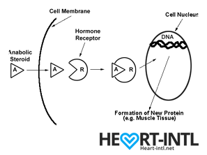
Let’s start with the working of hormones in our bodies.
Hormones are among the most important chemicals secreted in our bodies with each one having a very unique function.
Think of each hormone like a chemical messenger that carries a very specific message to our cells. Each cell in turn has a hormone receptor that receives this message and relays it to the cell to execute that command.
Anabolic Androgenic Hormones or Androgens
Testosterone
Testosterone, also known as the male hormone, belongs to a group of hormones called Androgens, that are associated with both anabolic and androgenic functions.
It helps you gain muscle (anabolic) but also helps you grow body hair and deepens your voice during puberty (Androgenic)
 Androgens
Androgens work in different ways in your body.
- They may directly bind to Androgen Receptors on the cells
- Convert into DHT (Dihydrotestosterone) and then may bind to androgen receptors on the cells
- Get converted into the hormone estradiol or estrogen, which then binds to a different type of receptor on cells called the estrogen receptor.
In normal circumstances, your body is primed to automatically regulate the production of androgens. It will only produce as much as you need to function normally.
But normal isn’t enough for bodybuilding. So, bodybuilders look for external sources of androgens, which are called anabolic steroids.
Anabolic Steroids
When you inject an anabolic steroid, your body has a sudden overload of androgens which saturate all androgen receptor cells. Each receptor then carries this response to the cells inducing both anabolic and androgenic changes.
Are we still on the same page? Hang on. It will be over soon.
Now, after saturating your cells, the body still has an excess of androgens that it cannot use.
So, it goes ahead and converts some of it into estrogen and you start to experience some of the unpleasant estrogen related side effects like bitch tits.
Some of the excess androgens might also get converted into DHT which will shrink your hair follicles causing hair loss. (Learn how N2Shampoo combats this.)
Some of these side effects, like the shrinking of your testes are temporary and can be reversed once you discontinue using steroids. However, some of the changes, like hair loss, cardiac problems and liver disease are permanent. That’s the tradeoff that you make for a better looking body.
Also, once you use an anabolic steroid, the chances of you getting hooked or dependent on them are extremely high.
Let’s face it man. You’ll love juice. Your energy levels are high. You look insanely ripped. You have bulging biceps, veins ready to pop out of your body. Your morning wood is strong enough to drill a hole in the wall with.
You will use steroids again. That’s a given and therein lies the risk.
SARMS
SARMS on the other hand, are non-steroidal and tissue selective in their action.
In other words, they carry only anabolic messages to androgen receptors in bone and muscle cells. They completely bypass cells associated with androgenic functions. So, your liver is spared the horror, your hair follicles will thank you and your heart will pump longer.
Steroids are like flooding your system with hormones that will give you 50% benefits and cause 50% damage. To curb or limit the damage, you will have to pop a hundred other pills like liver supplements and aromatase inhibitors.
SARMS will only target the cells that matter. It will relay the message to your muscles to start growing or your body to start burning fat. All the other irrelevant bull crap is ignored.
And it does it in two different, very interesting ways which we just briefed upon.
- It will attach itself only to muscle and bone tissue cells. Your other vital organs like liver and prostate are completely untouched.
- It doesn’t get broken down into other compounds like Estrogen and DHT which cause some of the worst side effects associated with steroid use.
The most important part here is the second one.
By not getting converted into 5-a reductase, an enzyme that is notorious for converting testosterone into DHT, it prevents most of the side effects associated with DHT. This makes SARMS the perfect stack to use with any androgenic steroid cycle.
SARMS also don’t shut you down completely. There will be testosterone suppression. But it’s not a complete shutdown. This allows you to recover sooner as compared to a steroid cycle where recovering from the shutdown might take weeks.
What are the benefits of using SARMS from an athlete’s or a bodybuilder’s perspective?
As we said earlier, SARMS were originally researched and developed for its therapeutic benefits in preventing conditions like cachexia, which accounts for at least 20% cancer related deaths.
But their usage in bodybuilding and professional sports is for entirely different reasons.
- Many bodybuilders and athletes do not want to use steroids for obvious reasons. SARMS allows them to dip their toes into synthetic compounds without risking it with steroids. It gives them a rough idea of what to expect, were they to go the AAS route. And the results are way better than using health supplements and multi vitamins.
- Others who are already using anabolic steroids, use SARMS to amplify the effects of their cycle while minimizing the sides. No DHT conversion, remember?
- The ability of SARMS to prevent muscle wasting helps in retaining lean muscle mass during a cutting cycle. There is no bloating due to water retention. Just plain, hard muscle.
Which are the best SARMS for various bodybuilding goals?
At some point of time during your journey to learn more about SARMS, you’d have this curiosity to know which the top five or ten SARMS are. But that’s a very difficult question to answer and a subjective one at that.
The best SARM for cutting may not be the ideal one for bulking and so on and so forth.
Nevertheless, we will list the most popular or widely used ones for you.
We are painting with a broad brush here mind you. But this will help you gain some perspective about which compound does what.
S4 – GTX007 –Andarine:
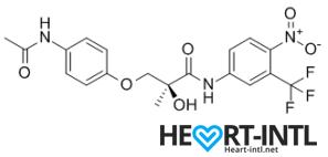
Chemical Structure of Andarine (S4)
Any bodybuilder or SARM user worth his salt would rave about S4. This is a first generation SARM that’s renowned for its ability to break through lifting plateaus. In simple terms, it will give you massive strength gains. But that’s not all. S4 also improves bone density, helps you gain lean mass, helps burn fat faster and helps your body recover sooner.
Is there anything it can’t do? S4 is also one of the best SARMs to stack with other SARMs, as well as with anabolic steroids. It’s a dream compound that should be a part of every stack to be honest. One of its innate abilities is to boost your libido and reduce spermatogenesis. So, if you thought that SARMs dipped your fertility levels, S4 is your best bet. It is very female-friendly as well (No masculine side effects) and is comparable to Anavar in giving users the ripped, venous look.
-
Lean Muscle Mass Gain
-
Fat Loss Acceleration
-
Strength Gain
Ligandrol – LGD-4033:
Ligrandrol is fondly called Anabolicum. That sort of sums it up, doesn’t it? If you wanted a SARM that was closest to Testosterone in its effects, then Ligandrol is just what you need. This immensely useful compound can help you pack some solid lean muscle in very little time. It is also associated with freakish strength gains and the ripped venous look that’s commonplace with Test-E usage. Zero water retention. Boosts your libido and overall wellbeing also.
-
Pumps
-
Lean muscle mass gain
-
Strength gain
-
Fatloss
Cardarine – GW-501516:
Cardarine is the ultimate cutting compound that should be in every body re-comp and cutting stack. It enhances gene expression and allows the body to tap into your stored fat reserves. Struggling to shed the jelly belly? Cardarine is your best bet. Additionally, it speeds up recovery and improves endurance.
-
Fat Loss
-
Energy
-
Improved endurance
-
Bigger Muscles
-
Versatility
Ostarine – MK-2866:
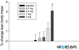
Lean Body Mass % change from baseline to day 86/End of Study
In the bodybuilding community, Ostaine is known as the recovery SARM. And hence, it always finds a place in every stack. But its benefits go way beyond muscle recovery. Ostarine earns the distinction of being one of the only SARMS to have undergone multiple clinical tests. All of which revealed an increase in lean muscle mass and reduce tissue degeneration. It is anabolic even in extremely low doses. Most bodybuilders use as much as 25mg/day for bulking cycles.
-
Lean muscle Gain
-
Energy
-
Muscle retention
Nutrobal (MK 677):
Nutrobal or MK 677 is a GH secretagogue that will boost your body’s natural production of Growth Hormone. This makes it one of the best SARMS to add to a PCT, following a steroid cycle. You are just experiencing the crash after a test overload and your body is raring to shed all that extra muscle that it gained. Nutrobal will help you retain that muscle without expensive HGH injections. Recommended dose is 25 mg/day.
-
Better Skin
-
Lean muscle gain
-
Fatloss
-
Better Sleep
Testolone (RAD140):
Testolone or RAD140 is one of the most researched compounds in the ever-expanding SARMS universe. Clinical studies have shown remarkable promise in helping prevent cancer cell division with RAD140. In the bodybuilding circuit, it is often compared with Primabolan, one of the safest steroids ever that was touted to be the favorite of the Austrian Oak himself. So, you are looking at safe, sustainable lean muscle gains, minimal water retention and almost zero sides.
-
Pumps
-
Lean Gains
-
Sense of Well Being
-
Strength Gains
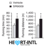
Stenbolic (SR9009):
Visit the link to read the full review on SR9009. We will discuss a study in depth which will give you some insights on what this powerful sarm is capable of.
-
Increased Metabolism
-
Fat Loss Acceleration
-
Improved Endurance
-
Muscle hypertrophy
SARMS vs. Anabolic Steroids
There are some very important differences between a SARM and a steroid beyond their mode of action in the body.
Steroids
An anabolic steroid instantly primes your body for just one sole purpose, to gain muscle.
Your protein synthesis skyrockets. Your energy levels peak. You are stronger than ever.
Your fat burn is accelerated and you will gain muscle when you lift, eat, sleep, walk, poop, have sex, irrespective of whether you eat right or not.
Think about your body as a machine that is designed to pack on as much muscle as it can, 24/7.
 The physical changes will be dramatic. The mental clarity will be amazing. It will help you break your plateau, it will help you crush your competition in sporting events (Lance Armstrong and even Michael Phelps?).
But, while doing all this, it will silently wreak havoc with your hormonal systems. The endocrine system takes the brunt. So do your liver and your cardiac muscles. Your balls shrink to the size of nuts. Your hair falls out in clumps. You develop bitch tits.
More often than not, the damage is irreparable.
Steroids are addictive. You will use again and your body builds a resistance to it. So, you will have to increase your dosage and add multiple compounds to your cycle. Before you even realize, you will be experimenting with at least three to four extremely dangerous compounds per cycle to keep your body looking the way it does.
And the side effect list is elaborate.
- Steroids can potentially enhance your risk of prostate cancer
- Steroids can give your permanent hair loss
- You can develop scar-causing cystic acne
- You will grow unwanted body hair
- Hypertension
- Permanent liver damage
- Cholesterol imbalance
- Left Ventricular Hypertrophy (Linked to multiple steroid related deaths)
SARMS
Compared to steroids, the effects of SARMS are not half as dramatic.
You will gain lean muscle. But you will have to consistently use SARMS for weeks before you see serious gains.
If you are a woman using SARMS, you won’t sprout a beard or develop a clitoris the size of a penis.
You will lose fat while gaining muscle, which again is one of the most sought after goals for body re-composition. The caveat is that the time frame taken for you to see results will be much longer.
Is that a bad thing? Not necessarily, because SARMS will not cause any of the toxicity that steroids cause.
We’d take an extended usage period any day in exchange for life threatening side effects. What about you?
Benefits of SARMs
Here are some of the typical benefits associated with SARMS:
- Works exactly like testosterone does
- Allows you to retain your hard earned muscle, even in a catabolic stage (Study)
- Helps you gain lean muscle while bulking with zero water retention
- Breaks your lifting threshold
- Your body recovers faster after a grueling workout
- Helps prevent joint pain (Study)
- Prevents cancer cell division (Study)
- Boosts libido
- Does not convert to DHT (Study)
- Does not breakdown into Estrogen
- It won’t suppress your HPTA (Hypothalamus-Pituitary-Testes-Axis) like steroids do
- Are not scheduled drugs. Steroids are Schedule III drugs which are illegal to procure and sell
- Some of the SARMS are undetectable in blood tests
- Are not liver toxic
- Are neuroprotective (Study)
One of the most amazing benefits of SARMS usage is that you do not need to prick needles to administer them.
Due to the legal status of steroids, many bodybuilders self-administer it and the only viable way to do it is the intramuscular way.
We are all aware of the potential risks of pricking the needle in the wrong place. Can even cause a paralytic attack. Not to mention the risks that come with needle sharing, which is rife in gyms.
SARMS help you avoid all these hassles.
Are SARMS Safe?
Coming to the big question, how safe are SARMS?
We’ll be brutally honest here. We just don’t know enough to say that its 100% safe.
We wish we could say that. But we aren’t here to peddle lies.
SARMS are still in their infancy. They have been studied and researched only for the past couple of decades and most of the research has been limited to rodents.
For the uninitiated, we share 98% of our DNA with rodents. But at the end of the day, we aren’t rats. So, for now, we just don’t know the long term effects of some of these compounds.
What we do know is that all the research conducted on rodents have been incredibly positive.
There have been a couple of human studies that have also been extremely positive.
But that’s clearly not enough, is it? We’d wait another fifty years to confirm what athletes and bodybuilders already know.
Aah!
Here’s what we do know apart from the benefits that we’ve listed above.
SARMS wont suppress your testosterone production as much as steroids do:
If you come across any website that claims that SARMS wont suppress your body’s natural testosterone production, skedaddle. SARMS will suppress you.
But the suppression won’t be as severe as taking external test-e. And hence, your testes wont shrink to the size of peanuts.
In one of the studies, males who were administered 3mg of Ostarine per day for 86 days were reported to have a 46% dip in their total testosterone levels. That’s almost 54% lesser than what external test does. But hey, it’s suppression nevertheless.
And the severity of the suppression increases with the amount of SARMS you use. If you are stacking, you are more likely to experience more suppression.
SARMS will cause some mild side effects:
It would be a fallacy to believe that any chemical compound that mimics the action of steroids in your body does not cause side effects.
SARMS will cause side effects. It’s just that in recommended doses and time frames, the side effects are usually too mild to become bothersome. We will come to this in a bit.
You will recover sooner from SARMS usage:
Because they don’t suppress you badly, you can recover a lot sooner from a SARMS cycle as compared to a steroid cycle.
Remember, they don’t convert to DHT or Estrogen as easily. So, you will be using fewer pills in your PCT. Many bodybuilders don’t even recommend a PCT with some SARMS.
SARMS may prevent cancer:
There have been some very controversial and contradictory reports about SARMS and cancer. There are a bunch of people who vehemently oppose the fact that SARMS have been known to inhibit cancer cell division. (Check the link to the clinical study provided above)
They cite a clinical study involving rodents that used ten times the recommended dose for five times the recommended time frame, as a reference to claim that SARMS can increase your risk of cancer. The keyword here is the dosage and the cycle time. Take ten times the recommended dose of Trenbolone in a day and please send us an advance invitation for your funeral the next day. Anything in excess is harmful. Be it SARMs or an OTC NSAID.
Unless more clinical studies are conducted at the recommended doses, we’d take the cancer warning with a pinch of salt.
Are SARMS legal?
Yes. They are. Surprising, isn’t it?
If you check the product label for SARMS, you’d notice a tiny warning message that says ‘Not for human consumption’. That’s precisely the loophole that allows manufacturers to sell SARMS legally over the counter.
According to the manufacturer, it’s just an experimental drug that’s not intended for human use. Yeah, right!

Elena Lashmanova
However, SARMS are bad news for professional athletes. They have been banned by WADA (World Anti-Doping Agency) since 2008. They have far too many muscle and bone specific anabolic properties that warrant abuse in professional sports. Quite a few athletes who sprung a new stride in their performance were caught using SARMS already. (Valery Kaykov, Elena Lashmanova)
So, they are listed under ‘other anabolic agents’ in section S1.2 in the prohibited list.
Are there any known side effects that may occur with SARMS use?
Yes. There are some possible side effects that may occur with SARMS use. However, most of these side effects have been noted at doses that are way beyond the recommended levels.
For example, the maximum recommended dosage of Cardarine (GW1516) or Endurobol is 10 mg/ml per day. But many bodybuilders use as much as 50 mg/ml a day. That’s an insanely high dose that speeds up the effects of the SARM. Subsequently, it may also cause some side effects.
Mild Virilization
One of the biggest draws of SARMS for female athletes and bodybuilders is that it does not cause virilization, or masculine features, which is commonplace with steroid use. However, virilization was noticed in some female bodybuilders when they overdosed on SARMS for a cycle period that was way more than the recommended usage time frame. Once again, the important point here is that the side effect was noted when the user consumed way more than what was recommended. If they’d used steroids in such high doses, they’d probably have died. In normal doses SARMS is considered to be safer than Clenbuterol, which is the favorite steroid for female athletes and celebrities.
Hairloss
Some bodybuilders who were genetically predisposed to balding noticed hair loss when they used SARMS. But it was nowhere as pronounced as the hair loss that occurs with steroid usage. SARMS are not androgenic and they do not break down into DHT. So, if you are likely to lose hair, SARMS may in fact be a much safer bet than using Anadrol or Dianabol which can make you go bald in weeks.
Gynecomastia
We know what you are thinking now. Don’t worry. SARMS don’t cause gynecomastia in 90% of the users. But there are a few who are extremely sensitive to estrogen. And in high doses, there can be a slight estrogen spike which is more than enough to trigger sensitive nipples in such users. Please remember that SARMS can have as much as a 90:10 anabolic to androgenic ratio. It is completely safe to use and rarely causes bitch tits. Even if you feel that your nipples are sensitive, mild doses of Nolvadex should suffice to curb it.
Vision problems
Mention SARMS and half of the internet will go for your throat citing that it can make you go blind. That’s far from the truth. Some SARMS have been associated with vision problems. In particular, it causes a yellowish tinge to your vision. This side effect that has spread like wildfire on the internet was first noticed with the usage of a SARM called Ostarine, once again in high doses. Also, it was noticed in only a handful of users. More importantly, the vision problems subsided automatically once usage was discontinued. Sadly, it is sporadic cases like these that gain more precedence over the hundred other beneficial effects of SARMS.
How to use SARMS
SARMS are extremely convenient and easy to use. They come in pocket-sized vials that can be tucked into your kit or even a messenger bag. There’s a doser in the bottle that takes the guesswork out of dosing.
You can just pop them into your mouth anytime you feel like.
- Squirt a measured dose into your mouth and swallow it. It’s usually tasteless. But if you are concerned about your taste buds, chase it down with a glass of juice. Thankfully, there are no restrictions about the variety of juice.
- Add the SARMS to a glass of juice or a can of your favorite energy drink gulp it down.
After speaking to several experienced SARMS users, we found that the second method works best. It prevents you from tasting the compound and you can choose your favorite juice or energy drink to mix it with.
How not to use them
Because of their similarity to anabolic steroids, a lot of users misinterpret the right way to take SARMS. And they use it like they administer steroids.
- Sublingually: Many testosterone boosters, secretagogues and even some steroids are administered sublingually, that is by placing the dose under the tongue until it is absorbed into the bloodstream. But SARMS must not be taken sublingually because they tend to burn the sensitive skin under the tongue. It’s just a slight warm feeling. But why administer it that way when there’s an easier way to use it?
- Injections: Any research chemical is intended for oral administration only. They are not sterilized for intramuscular injections. So, never inject a SARM.
- Transdermal patches: As far as we know, there are no SARMS available for transdermal application. However, some users have mixed them with Dimethyl sulfoxide (DMSO), creating a DIY transdermal patch. We don’t recommend this one bit. Just drink the damn cocktail will you?
Can you stack SARMS?
Absolutely! Their limited androgenic effects and few side effects make them excellent chemicals to stack together to achieve your bodybuilding goals. However, to ensure that you maximize your results and minimize the risk of mild side effects, we recommend that you stack SARMS that complement each other rather.
Here are a few stackable SARM combinations.
S4 with any SARM
S4 is one of the oldest SARMS to be discovered and hence, it is also among the most widely used ones. Most users recommend pairing it with another SARM, like MK-2866 or Ligandrol for maximizing its benefits. However, stacking multiple SARMS together increases your risk of testosterone suppression.
Cardarine and Ligandrol
Cardarine or GW1516 is one of the most promising compounds to have come out of the SARMS stable. It is known to amplifiy gene expression and even touted to help build mitochondria in the body, which is nothing short of amazing. Having said that, such a potent compound must be dealt with caution. So go slow with your Cardaine intake and stack it with Ligrandrol for best results.
Ostraine and Ligandrol
Ostraine is one of the safest SARMS ever. Its side effects are limited to very mild testosterone suppression. This makes it one of the best SARMS to stack with others. Ligrandrol makes for a very compatible stacking compound with Ostarine. You can expect excellent lean muscle gains clubbed with noticeable fat loss on this stack.
Ostarine & Cardarine
This is the perfect body re-composition combo stack. It helps improving lean muscle gains while amplifying fat loss and also improving strength gains. Ostarine does the bulk of the lifting here. But it is also associated with some side effects like elevated Estrogen levels (In sensitive users) and it may also suppress the HPG axis mildly. At least, some of these side effects can be negated with Cardarine.
Andarine, Cardarine, Ostarine
This is the ultimate cutting stack. We already spoke briefly about Ostarine, the do-it-all compound. Let’s talk about the other two in this stack. Cardarine is technically not a SARM. Instead, it is a compound that is very similar to a SARM that activates an enzyme called AMPK, that helps the body burn stored fat. If initial reports are to be believed, it might play a key role in the prevention of Type-II diabetes. Lastly, you have Ardarine, which helps improve bone density and strength, which can get depleted during a cutting cycle. As we said, this stack will significantly improve your goals during a cutting cycle.
Can you stack SARMS with Steroids?
The right question would be whether you ‘Should’ stack SARMS with steroids.
The answer is a big, resounding Yes.
There are numerous ways in which SARMS can help.
They can negate some of the side effects of steroids. They can amplify some of the beneficial effects of steroids.
In simple terms, we’d never attempt a steroid cycle without adding SARMS to it.
Here are some of the obvious contenders.
GW501516 – Best used with Trenbolone – Can help reduce the cholesterol and blood pressure spikes that come with Tren use.
SR9009 – Helps boost cardiovascular strength and prevents joint problems associated with Tren and Deca.
MK2866 – Helps your body recover during PCT and also helps reduce cortisol levels which in turn can eat away on your hard earned gains. Add it to your Test-E and Winstrol cycle.
Conclusion
Move aside needle-heads. We have a newer and safer drug on the horizon.
One that doesn’t shrink balls or blunt your hormone production.
SARMs have shown tremendous promise in the field of medicine and performance enhancement. With its selective tissue based action and minimal androgenic effects, there is no reason why it might replace AAS or steroids one day.
What is your experience with SARMS? Have you used any of these compounds or stacked them? We would love to hear about it.
Thank you for one of the most comprehensive explanations of the various SARMS that I have found.
I am currently taking a combination of 30IU’s per day (2Xinjections) and was wondering about supplementing this with SR9009. I am after muscle increase and fat loss. I am also 77 years of age but look about mid fifties. I am also a gym junkie and go ,on average, five times per week.
I hope that you will respond to this email
I am interested in your products, how much is it? and how can i get them?
You can buy sarms from sarms1.com
how to use them effectively
how can i use them effectively
How sustainable are these gains? I know we need to stop for a few weeks and then go again, but I am hoping to get to my goal and then stop completely 100% and not trying to touch it again, and will go natural and clean to maintain it. But hate to see the loss of what I gained through natural diet, and hence my question if I need to do this stack or cycle for 2-3 cycles or forever or one is enough, if followed with super clean and discipline workout and diet.
You will keep the gains if you do a proper PCT and use SARMS Support with your (and after) cycle.
Generally Clomid/Nolvadex with HCGenerate ES or POST CT. Stacked with Stenabolic (SR).
wow this is comprehensive information. everyone should save this and use it as a reference
sarms are really effective